R on Android

In Riyadh I spent a rainy afternoon trying to work out how this was done (no, not really rainy but stayed indoors instead of driving about the desert). There's not much on the web about it. For at least a year people have been saying there will be an app - and yes, one will eventually appear, but for now this is how we can get our kicks.

rwiki says that it's easy to install R on Android but it needs a lot of patching (so perhaps not so easy after all).  

At LinkedIn (may need to subscribe to see this) a couple of clues from clever geeks said things like:
"...Just set up an Rstudio server using an Amazon instance and be done as you can use it from any internet connection"
and:
"You could run r in an amazon aws instance (a micro instance is free right now for limited hours / month) and access that from a tablet or computer if you use r studio server. The advantages are that - works on any platform..."

So how can you do this on Amazon AWS (Amazon Web Services)? It must be so easy but the geeks don't say - and it's free.  Never having used these services before, one becomes easily overwhelmed by the sheer number of services on offer - which one to choose? See: http://aws.amazon.com/free/

I set it all up on my laptop first (running Windows).

You should choose Amazon EC2 (Amazon Elastic Compute Cloud). You will need to click on the Get Started for Free button, you need to register a credit card. 

Once you are registered you should be able to select a console page. If not, go here:https://console.aws.amazon.com/console/homeand click on the icon for EC2

This gives me the EC2 dashboard. For some reason I have been allocated resources at US West (Oregon), and yet I am in Saudi Arabia. Hopefully you will find a nearer more appropriate allocation (or maybe it just doesn't matter).  From here you want to Launch Instance.

You will find the instructions in this youtube video most helpful for the rest of setting up the EC2:http://www.youtube.com/watch?NR=1&v=OLfmqcYnhUM

A floating window appears Create a New Instance. Click Continue (Classic Wizard).
A dazzling range of AMIs (Amazon Machine Images) are available. I selected the Microsoft Windows Server 2008 Base 64 bit (starred indicating it is free).

As suggested in the video select the default settings.
From the Windows Start button search for Remote Desktop Connection to launch the server window. From the floating window that comes up when you connect, you should copy & paste the DNS address (this is different each time you make a connection). You need to type in Administrator and the generated password - as seen in the video (generating the password may take a while, 15 or more minutes, keep refreshing to check).
Once you are in to the Windows server run Explorer and install R from CRAN. 

While in Windows I found it useful to change my password to something more memorable.When finished, Logout. Back in normal Windows you should Stop the instance. Your usage will then stop. Important: do not Terminate or this will remove the instance completely (R installation and all).

Go to android phone. 

Install a remote connection client app, I tried 2X Client RDP/Remote Desktop which works very well and is free.

Update:
It is well worth installing the AWS Console app on the phone. This makes it much less fiddly stopping and starting the instance. For some reason the default is for Virginia, so you may need to change the area. 


Run web browser. Go to the EC2 Management Console page, as seen earlier on laptop. You should see the instance that you set up, and it should be in a stopped state (assuming you stopped it earlier).Select the instance, and from the Actions menu click on Start, confirm Yes on floating window.It will show pending and changing quite soon to show running.From the Actions menu select Connect. This will give you the login information and you need to copy and paste the Public DNS from here. 

Run the 2X Client, choose an RDP connection, then:
1. paste Public DNS into the Server
2. enter Administrator for name (if local network specifies its own domain then enter amazon\Administrator instead)
3. enter password from before
4. Select Connect to Console
5. Connect, click on icon next to X, then select item

After a few seconds delay, you should see the screen below (as on my Samsung Galaxy SIII). There is a dinky mouse with pointer (shown in center of screen) and a keyboard. Extra characters are available by selecting Shift.

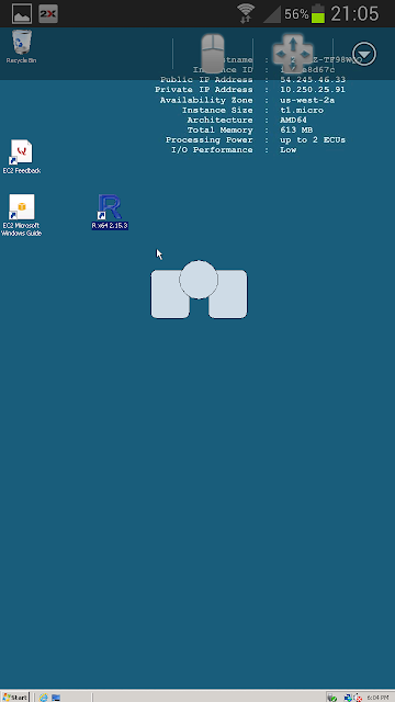
Running R gives the screen below. Very small and fiddly - but definitely worth it!

Once you have logged out, remember to stop the instance else you could run up charges (it may be hard to find the floating window asking for Yes confirmation of this). 

After this my usage report (downloaded CSV) looked massive...But Account activity = £0.0

Perhaps on another rainy afternoon I'll set up RStudio for my phone.

Using RExcel for Likelihood Ratios

The likelihood ratio (Law of Likelihood) provides a measure of the relative strength of evidence for competing models/hypotheses given the observed data. Richard Royall has championed this approach, e.g. this paper. A paper by Scott Glover & Peter Dixon (2004) nicely illustrated the use of likelihood ratios in regression and ANOVA. Likelihood ratios give much more flexibility than the usual null hypothesis testing approach. They allow you to ask very specific questions about your data.

Likelihood ratios near 1 indicate that insufficient data have been collected, while a ratio of 4 represents "weak" evidence, 8 is "fairly strong", 32 is "strong". There is no cut-off value like the .05 used in null hypothesis significance testing.

The likelihood ratio:

Since the likelihood for a model is inversely related to the residual (G&D paper gives the proof), we get the following:

Where R² is the amount of variance explained by each model and N is the total number of observations. This gives:

The likelihood ratio (LR) can also be obtained from the Akaike information criterion (AIC) that is produced by R statistics for model comparison:

AIC = -2ln(L) + 2k

The likelihood ratio is simply available by:

λ = exp((AIC₂ – AIC₁)/2)

The AIC method takes into account model complexity (number of parameters) while the R² method doesn't. However, both methods require applying a correction for small samples. Note that at least 2 of the formulae given in the G&D paper for this correction have simple errors. For corrected LR using R² see the G&D paper, and for AIC see http://en.wikipedia.org/wiki/Akaike_criterion under AICc.

Excel and RExcel Workbook (click here to download)
The Excel workbook here has 3 different sheets, each of which incorporate calls to R through RExcel. All cells are locked except those that are intended to be altered manually, but can be unprotected (from Review menu) without a password. Select automatic under Calculation Options so that any changes are automatically re-calculated.

Regression models
The first illustrates the example from the G&D paper on comparing a linear to a quadratic regression fit to the same data - see the plots below.  

The data are similar, but not identical, to that used in the paper. The values in the X & Y data columns can be changed - which results in immediate recalculation of all the LRs, the plots & fits etc (this is the joy of using RExcel). 

2-way ANOVA
The next sheet uses some data that I use in teaching 2-way ANOVA, the so-called "Beergoggles" example (the more drunk males are the more attractive they find others). The sheet calculates the LRs for specific hypotheses. The first hypothesis compares an interactive model (where we assume there is an interaction) with an additive model (main effects only). The LR of 123 is strongly in favour of an interactive model. 

The second hypothesis compares a specific contrast. Contrasts are easily calculated using:

where n is the number in each ith condition, X̅ is the mean and c is the contrast coefficient for each condition. In the sheet the contrast consisting of the drunk male group (8.36) vs the remaining 5 conditions is compared with the full model (main effects + interaction). The LR value of 3.76 here represents weak evidence that the contrast is a better model than the full model. (Note, none of the values in this sheet can be altered, all cells locked).

t test and specified effect
The final sheet shows a t test where the means and SDs for the two groups can be chosen and random normally distributed data generated in the data (BP - diastolic blood pressure in hypertensive patients) column. Pressing F9 generates new random data, and new statistics automatically re-calculated. R calculates the p value in the ANOVA summary table, and LR is calculated for the model that includes a difference in conditions against the null model. The first λ_C is the LR in favour of the difference model, while its inverse below it is the LR in favour of the null model. A small p value will produce a small value for the latter.

Below this the λ_C is for a specific value for the drug effect (e.g. 86 mmHg) versus the null model. This value might be the expected drug effect or the minimal drug effect of clinical importance. Note that the two models have the same number of parameters (2: the mean and variance). 

To the right of the sheet is shown the minimum Bayes factor and a range of posterior probabilities for the null according to prior odds. This will be explained in a future post.


Conclusion
The use of LRs is a flexible approach to assess the strength of evidence for one model over another. It is not subject to the same difficulties encountered by p values in null hypothesis significance testing, such as multiple testing, stopping rules, and planned vs unplanned tests. Finally, the LRs from different studies can be combined by simply multiplying them together. 


References:
Glover, S., & Dixon, P. (2004). Likelihood ratios: A simple and flexible statistic for empirical psychologists. Psychonomic Bulletin & Review, 11(5), 791-806. or available at doi:10.3758/BF03196706

Which side are you on?

Problems with orthodox statistics
Zoltan Dienes has written an interesting and stimulating paper in support of Bayesian inference over orthodox Neyman-Pearson/Fisherian inference. The paper is based upon his 2008 book (book reviewed by Baguley & Kaye (2010)). In his book Dienes had favoured the Likelihood approach, but in this paper he appears to have moved much further to supporting the Bayesian approach. Dienes writes well: and it's worth reading the book that fleshes out issues briefly mentioned in the paper.

The issue of over-reliance on p values contrasts with confidence interval and effect size approaches (see for example Ziliak & McCloskey (2008) and Meehl (1978)). Dienes attempts to show that orthodox inference is inconsistent & flawed, and that we have no choice but to do things differently. The issues run deep and are mired by a long history of controversy.

In his paper Dienes gives 3 research scenarios as follows, and I quote:

1. Stopping rule
You have run the 20 subjects you planned and have obtained a p value of .08. Despite predicting a difference, you know this won’t be convincing to any editor and run 20 more subjects. SPSS now gives a p of .01. Would you:
a) Submit the study with all 40 participants and report an overall p of .01?
b) Regard the study as nonsignificant at the 5% level and stop pursuing the effect in question, as each individual 20-subject study had a p of .08?
c) Use a method of evaluating evidence that is not sensitive to your intentions concerning when you planned to stop collecting subjects, and base conclusions on all the data?


2. Planned versus post hoc
After collecting data in a three-way design, you find an unexpected partial two-way interaction, specifically you obtain a two-way interaction (p = .03) for just the males and not the females. After talking to some colleagues and reading the literature, you realize there is a neat way of accounting for these results: Certain theories can be used to predict the interaction for the males but they say nothing about females. Would you:
a) Write up the introduction based on the theories leading to a planned contrast for the males, which is then significant?
b) Treat the partial two-way as nonsignificant, as the three-way interaction was not significant, and the partial interaction won’t survive corrections for post hoc testing?
c) Determine how strong the evidence of the partial two-way interaction is for the theory you put together to explain it, with no regard to whether you happen to think of the theory before seeing the data or afterwards, as all sorts of arbitrary factors could influence when you thought of a theory?


3. Multiple testing
You explore five possible ways of inducing subliminal perception as measured with priming. Each method interferes with vision in a different way. The test for each method has a power of 80% for a 5% significance level to detect the size of priming produced by conscious perception. Of these methods, the results for four are nonsignificant and one, Continuous Flash Suppression, is significant, p = .03, with a priming effect numerically similar in size to that found with conscious perception. Would you:
a) Report the test as p = .03 and conclude there is subliminal perception for this method?
b) Note that all tests are nonsignificant when a Bonferroni-corrected significance value of .05/5 is used, and conclude that subliminal perception does not exist by any of these methods?
c) Regard the strength of evidence provided by these data for subliminal perception produced by Continuous Flash Suppression to be the same regardless of whether or not four other rather different methods were tested?

Most active researchers will have personally encountered these scenarios. To each of the 3 scenarios: choosing option a) is the temptation that many researchers succumb to, and is wrong. Choosing b) is what you should do if you adopt a disciplined Neyman-Pearson approach (as he says "maybe your conscience told you so"). Finally choosing c) appears to be the most desirable and can only be implemented using a Bayesian approach.

The Likelihood
It is claimed that the orthodox answers (b) violate the likelihood principle and hence the axioms of probability. Well, what is the likelihood principle? It is: "All the information relevant to inference contained in data is provided by the likelihood."

The likelihood ratio which represents the relative evidence of one theory over another has been elevated to the "Law of likelihood", as coined by Hacking (1965) (a difficult book, not recommended). Basically then, this states that the actual data obtained most strongly supports the theory that predicted it. The strong likelihood principle can be applied to sequential experiments (e.g. Armitage et al (2002), p615).

The likelihood is a relative probability, and differs from the p value. The p value is the probability of obtaining the data or more extreme data, given a (null) hypothesis and a decision procedure. It is an area under the probability curve. In contrast, the likelihood is the height of the probability curve at the point representing the obtained data. The strength of evidence (the likelihood) can be separated from the probability of obtaining the evidence (the relative costings of the two types of errors, α and β, in the Neyman-Pearson formulation). The p value in a statistical test combines and confuses the strength of evidence and the probability of obtaining that evidence - which is why we run into problems in the 3 scenarios above.

Bayesian approach using the Bayes factor
Bayesian methods aim to determine the probability of a theory given the data. The posterior odds is equal to the likelihood ratio multiplied by the the prior odds (the odds of the theory before data is collected). Rather than calculate the posterior odds, Dienes recommends calculating the Bayes factor. This is the ratio of likelihoods for the theory and the null (how much the data supports your theory versus the null). According to Jeffreys (1961) a Bayes factor greater than 3 or less than 1/3 indicates substantial evidence for or against a theory (a Bayes factor of unity represents no evidence either way and usually indicates low sensitivity - i.e. not enough data). With "moderate numbers" a Bayes factor of 3 corresponds roughly to the conventional 5% significance level. Effect size and shape of the prior distribution (typically uniform or normal) need to be considered in order to calculate the Bayes factor. Explicitly using effect sizes forces the researcher to think about and engage with the data in their research domain. As Dienes (2011) says: "People will think more carefully about theoretical mechanisms so as to link experiments to past research to predict relevant effect sizes. Results sections will become focused, concise, and more persuasive."

Extra data can be added at any time where the probability of producing a Bayes factor that is weak (close to 1). Misleading (wrong direction) Bayes factors decrease the more data there is. This is not true for p values or for the probability of making a Type I error. When the null hypothesis is true then p values are not driven in any direction (Type I error remains at 5%) as sample size increases, while the Bayes factor is driven to 0.

Conclusion
Dienes has written a persuasive paper. The recommended Bayesian approach should be explored and tried out by researchers, and is easier than previous suggestions (e.g. Berger, 2003). It will be interesting to see how successful authors are at getting it past journal reviewers. The Bayesian approach is intuitively appealing: it is much easier to think about a ratio of likelihoods for competing theories than it is to appreciate the probability of obtaining extreme data assuming the null hypothesis is true. One problem with Bayesian probability/factor calculation is that they currently appear awkward and complicated. Hopefully this will change in time and encourage researchers to think more about their data and the theories they support.

Addendum
Another interesting approach suggested by Goodman (1999) in which the minimum Bayes Factor for the null hypothesis is calculated directly from z, t or χ². This can be compared with the conventional p value, but more than that it informs us of the maximum decrease in the prior probability of a null hypothesis.

How to calculate a simple Bayes factor
Matlab code is provided at Dienes' website and is translated into R by Baguley & Kaye (2010) also available from Kaye's website. I reproduce it here formatted (and also because copying directly from the Baguley & Kaye (2010) paper didn't work for me). Here first is an Excel file containing 3 worksheets:
1) VBA macro with graphic, enter values into yellow cells and click on Calculate button. The graphic shows the position of the obtained mean, the null likelihood, the theory probability distribution (not taking into account the obtained data), and the product between the theory distribution and data likelihood. This latter product does not represent a probability density as such (but is plotted anyway and looks like the (diminutive) posterior probability distribution). The product values are integrated to provide the theory likelihood, p(D | Theory) - thanks to Zoltan Dienes for clarifying these issues (hoping I've got it right this time!)
2) RExcel where values for statistics & parameters can be entered in the yellow cells, and outputs automatically re-calculated by Excel (have it on Automatic calculation option. Follow the instructions in the green cells.
3) a sheet illustrating Goodman's minimum Bayes Factor.

All sheets are locked but can easily be unlocked without entering a password.

In the RExcel worksheet: After installing R and RExcel (Randfriends is the easiest way) you need to do the following:
1. Start R in Add-Ins RExcel menu
2. Select blue cell, remove ' (apostrophe) then press F2 and then Enter (this runs the function)
3. Select the 3 blue cells and in formula bar remove ' then Ctrl + Shift + Enter


Else the following code can be run in R directly:

Bf <- function(sd, obtained, uniform, lower = 0, upper = 1,

  meanoftheory = 0, sdtheory = 1, tail = 2)

{

#test data can be found starting at p100 of Dienes (2008) adapted from Baguley & Kaye (2010)

#

area <- 0

if (identical (uniform, 1)){

  theta <- lower

  range <- upper-lower

  incr <- range/2000

  for (A in -1000:1000) {

    theta <- theta + incr

    dist_theta <- 1/range

    height <- dist_theta * dnorm(obtained, theta, sd)

    area <- area + height * incr

    }

  } else {

    theta <- meanoftheory-5 * sdtheory

    incr <- sdtheory/200

    for (A in -1000:1000) {

      theta <- theta + incr

      dist_theta <- dnorm(theta, meanoftheory, sdtheory)

      if (identical(tail, 1)) {

        if (theta <= 0){

        dist_theta <- 0

        } else {

      dist_theta <- dist_theta * 2

      }

    }

    height <- dist_theta * dnorm(obtained, theta, sd)

    area <- area + height * incr

  }

}

LikelihoodTheory <- area

Likelihoodnull <- dnorm(obtained, 0, sd)

BayesFactor <- LikelihoodTheory/Likelihoodnull

ret <- list("LikelihoodTheory" = LikelihoodTheory,

"Likelihoodnull" = Likelihoodnull, "BayesFactor" = BayesFactor)

ret

}

Then the following commands can be issued:

Bf(1.09,-2.8,1,lower=-600,upper=0)
giving:
$LikelihoodTheory = 0:00166435
$Likelihoodnull = 0:01350761
$BayesFactor = 0:1232157

Bf(1.09,-2.8,0,meanoftheory=0,sdtheory=2,tail=1)
giving:
$LikelihoodTheory = 0:001955743
$Likelihoodnull = 0:01350761
$BayesFactor = 0:1447882

Bf(1.09,-2.8,0,meanoftheory=0,sdtheory=2,tail= 2)
giving:
$LikelihoodTheory = 0:08227421
$Likelihoodnull = 0:01350761
$BayesFactor = 6:090951

References:

Armitage, P., Berry, G. & Matthews, J.N.S. (2002) Statistical Methods in Medical Research. Oxford: Blackwell Science.

Baguley, T. & Kaye, D. (2010) Book review of Dienes' book, British Journal of Mathematical and Statistical Psychology, 63: 695–698. Available here: http://bit.ly/kq7iXh and R code available at: http://www.danny-kaye.co.uk/Docs/Dienes_functions.txt

Berger, J.O. (2003) Could Fisher, Jeffreys and Neyman Have Agreed on Testing? Statistical Science, 18(1): 1-32.

Dienes, Z. (2008) Understanding psychology as a science: An introduction to scientific and statistical inference, Palgrave Macmillan, Paperback, ISBN: 978-0-230-54231-0

Dienes, Z. (2011) Bayesian Versus Orthodox Statistics: Which Side Are You On? Perspectives on Psychological Science, 6(3): 274–290.

Goodman, S.N. (1999) Toward Evidence-Based Medical Statistics. 2: The Bayes Factor, Annals of Internal Medicine, 130(12):1005-13

Hacking, I. (1965) Logic of statistical inference, Cambridge University Press.

Jeffreys, H. (1961) The Theory of Probability, Oxford University Press.

Meehl, P. E. (1978) Theoretical risks and tabular asterisks: Sir Karl, Sir Ronald, and the slow progress of soft psychology. Journal of Consulting and Clinical Psychology, 46(4): 806-834.

Ziliak, S.T., & McCloskey, D.N. (2008) The cult of statistical significance: How the standard error cost us jobs, justice and lives, Ann Arbor: University of Michigan Press.

Matrix plot with confidence intervals for r values

The Iris data.
I like this way of plotting bivariate data, where histograms of the variables are given, and for the bivariate plots correlations with their 95% confidence intervals are displayed. The plots have LOESS curves.

Here is the R code:

## put histograms on the diagonal
panel.hist <- function(x, ...)
{
    usr <- par("usr"); on.exit(par(usr))
    par(usr = c(usr[1:2], 0, 1.5) )
    h <- hist(x, plot = FALSE)
    breaks <- h$breaks; nB <- length(breaks)
    y <- h$counts; y <- y/max(y)
rect(breaks[-nB], 0, breaks[-1], y, col="lavender", ...)
}
## put correlations & 95% CIs on the upper panels,
panel.cor <- function(x, y, digits=2, prefix="", cex.cor, ...)
{
    usr <- par("usr"); on.exit(par(usr))
    par(usr = c(0, 1, 0, 1))
    r <- cor(x, y,use="complete.obs")
    txt <- format(c(r, 0.123456789), digits=digits)[1]
    prefix <- "r = "
    rc <- cor.test(x,y)
    rci <- rc$conf.int
    txt2 <- format(c(rci, 0.123456789), digits=digits)[1]
    txt3 <- format(c(rci, 0.123456789), digits=digits)[2]
    prefix2 <- "\nCI = "
    txt <- paste(prefix, txt, prefix2, txt2, ", ", txt3, sep="")
    if(missing(cex.cor)) cex.cor <- 0.8/strwidth(txt)
    text(0.5, 0.5, txt, cex = 1)
}
pairs(iris[1:4], lower.panel=panel.smooth, cex = .8, pch = 21, bg="steelblue",
       diag.panel=panel.hist, cex.labels = 1.2, font.labels=2, upper.panel=panel.cor)

This is the R code used to produce the Motion Chart:

install.packages('googleVis')

library(RJSONIO)

library(googleVis)

M <- gvisMotionChart(Smoking, idvar="Disorder", timevar="Age", options=list(state='{\"showTrails\":false};'))

plot(M)

cat(M$html$chart, file="tmp.html")    #this produces html for pasting into blog

The table below is taken from Figure 4 of Woloshin et al (2008)

Grey shading means fewer than 1 death per 1000 women. All ratios are >= 0.75 (grey shaded data gave ratios of 1).

												Lung
		Vascular	Disease			Cancer				Infection		Disease
Age	Smoking status	Heart		Lung	Breast	Colon	Ovarian	Cervical						All
		Disease	Stroke	Cancer	Cancer	Cancer	Cancer	Cancer	Pneumonia	Flu	AIDS	COPD	Accidents	Combined
35	Never smoker	1			1						1		2	14
	Smoker	1	1	1	1						1		2	14
40	Never smoker	1			2	1					1		2	19
	Smoker	4	2	4	2						1	1	2	27
45	Never smoker	2	1	1	3	1	1				1		2	25
	Smoker	9	3	7	3	1	1		1		1	2	2	45
50	Never smoker	4	1	1	4	1	1						2	37
	Smoker	13	5	14	4	1	1		1			4	2	69
55	Never smoker	8	2	2	6	2	2	1	1			1	2	55
	Smoker	20	6	26	5	2	2	1	1			9	2	110
60	Never smoker	14	4	3	7	3	3	1	1			2	2	84
	Smoker	31	8	41	6	3	3	1	2			18	2	167
65	Never smoker	25	7	5	8	5	4	1	2			3	3	131
	Smoker	45	15	55	7	5	3	1	4			31	3	241
70	Never smoker	46	14	7	9	7	4	1	4			5	4	207
	Smoker	66	25	61	8	6	4	1	7			44	4	335
75	Never smoker	86	30	7	10	10	5	1	8			6	7	335
	Smoker	99	34	58	10	9	4		14			61	7	463

Here is the data (Smoking) based on the table and used by the R code:

Disorder	Age	Type	N_per_1000	Ratio
Heart Disease	2035	Vascular disease	1	1.000
Heart Disease	2040	Vascular disease	4	4.000
Heart Disease	2045	Vascular disease	9	4.500
Heart Disease	2050	Vascular disease	13	3.250
Heart Disease	2055	Vascular disease	20	2.500
Heart Disease	2060	Vascular disease	31	2.214
Heart Disease	2065	Vascular disease	45	1.800
Heart Disease	2070	Vascular disease	66	1.435
Heart Disease	2075	Vascular disease	99	1.151
Stroke	2035	Vascular disease	1	1.000
Stroke	2040	Vascular disease	2	1.000
Stroke	2045	Vascular disease	3	3.000
Stroke	2050	Vascular disease	5	5.000
Stroke	2055	Vascular disease	6	3.000
Stroke	2060	Vascular disease	8	2.000
Stroke	2065	Vascular disease	15	2.143
Stroke	2070	Vascular disease	25	1.786
Stroke	2075	Vascular disease	34	1.133
Lung Cancer	2035	Cancer	1	1.000
Lung Cancer	2040	Cancer	4	1.000
Lung Cancer	2045	Cancer	7	7.000
Lung Cancer	2050	Cancer	14	14.000
Lung Cancer	2055	Cancer	26	13.000
Lung Cancer	2060	Cancer	41	13.667
Lung Cancer	2065	Cancer	55	11.000
Lung Cancer	2070	Cancer	61	8.714
Lung Cancer	2075	Cancer	58	8.286
Breast Cancer	2035	Cancer	1	1.000
Breast Cancer	2040	Cancer	2	1.000
Breast Cancer	2045	Cancer	3	1.000
Breast Cancer	2050	Cancer	4	1.000
Breast Cancer	2055	Cancer	5	0.833
Breast Cancer	2060	Cancer	6	0.857
Breast Cancer	2065	Cancer	7	0.875
Breast Cancer	2070	Cancer	8	0.889
Breast Cancer	2075	Cancer	10	1.000
Colon Cancer	2035	Cancer	0	1.000
Colon Cancer	2040	Cancer	0	1.000
Colon Cancer	2045	Cancer	1	1.000
Colon Cancer	2050	Cancer	1	1.000
Colon Cancer	2055	Cancer	2	1.000
Colon Cancer	2060	Cancer	3	1.000
Colon Cancer	2065	Cancer	5	1.000
Colon Cancer	2070	Cancer	6	0.857
Colon Cancer	2075	Cancer	9	0.900
Ovarian Cancer	2035	Cancer	0	1.000
Ovarian Cancer	2040	Cancer	0	1.000
Ovarian Cancer	2045	Cancer	1	1.000
Ovarian Cancer	2050	Cancer	1	1.000
Ovarian Cancer	2055	Cancer	2	1.000
Ovarian Cancer	2060	Cancer	3	1.000
Ovarian Cancer	2065	Cancer	3	0.750
Ovarian Cancer	2070	Cancer	4	1.000
Ovarian Cancer	2075	Cancer	4	0.800
Cervical Cancer	2035	Cancer	0	1.000
Cervical Cancer	2040	Cancer	0	1.000
Cervical Cancer	2045	Cancer	0	1.000
Cervical Cancer	2050	Cancer	0	1.000
Cervical Cancer	2055	Cancer	1	1.000
Cervical Cancer	2060	Cancer	1	1.000
Cervical Cancer	2065	Cancer	1	1.000
Cervical Cancer	2070	Cancer	1	1.000
Cervical Cancer	2075	Cancer	0	1.000
Pneumonia	2035	Infection	0	1.000
Pneumonia	2040	Infection	0	1.000
Pneumonia	2045	Infection	1	1.000
Pneumonia	2050	Infection	1	1.000
Pneumonia	2055	Infection	1	1.000
Pneumonia	2060	Infection	2	2.000
Pneumonia	2065	Infection	4	2.000
Pneumonia	2070	Infection	7	1.750
Pneumonia	2075	Infection	14	1.750
AIDS	2035	Infection	1	1.000
AIDS	2040	Infection	1	1.000
AIDS	2045	Infection	1	1.000
AIDS	2050	Infection	0	1.000
AIDS	2055	Infection	0	1.000
AIDS	2060	Infection	0	1.000
AIDS	2065	Infection	0	1.000
AIDS	2070	Infection	0	1.000
AIDS	2075	Infection	0	1.000
COPD	2035	Lung disease	0	1.000
COPD	2040	Lung disease	1	1.000
COPD	2045	Lung disease	2	1.000
COPD	2050	Lung disease	4	1.000
COPD	2055	Lung disease	9	9.000
COPD	2060	Lung disease	18	9.000
COPD	2065	Lung disease	31	10.333
COPD	2070	Lung disease	44	8.800
COPD	2075	Lung disease	61	10.167
Accidents	2035	Accidents	2	1.000
Accidents	2040	Accidents	2	1.000
Accidents	2045	Accidents	2	1.000
Accidents	2050	Accidents	2	1.000
Accidents	2055	Accidents	2	1.000
Accidents	2060	Accidents	2	1.000
Accidents	2065	Accidents	3	1.000
Accidents	2070	Accidents	4	1.000
Accidents	2075	Accidents	7	1.000